Alfonso Zamora
Cloud Engineer

Introduction
The main goal of this article is to present a solution for data analysis and engineering from a business perspective, without requiring specialized technical knowledge.
Companies have a large number of data engineering processes to extract the most value from their business, and sometimes, very complex solutions for the required use case. From here, we propose to simplify the operation so that a business user, who previously could not carry out the development and implementation of the technical part, will now be self-sufficient, and will be able to implement their own technical solutions with natural language.
To fulfill our goal, we will make use of various services from the Google Cloud platform to create both the necessary infrastructure and the different technological components to extract all the value from business information.
Before we begin
Before we begin with the development of the article, let’s explain some basic concepts about the services and different frameworks we will use for implementation:
- Cloud Storage[1]: It is a cloud storage service provided by Google Cloud Platform (GCP) that allows users to securely and scalably store and retrieve data.
- BigQuery[2]: It is a fully managed data analytics service that allows you to run SQL queries on massive datasets in GCP. It is especially effective for large-scale data analysis.
- Terraform[3]: It is an infrastructure as code (IaC) tool developed by HashiCorp. It allows users to describe and manage infrastructure using configuration files in the HashiCorp Configuration Language (HCL). With Terraform, you can define resources and providers declaratively, making it easier to create and manage infrastructure on platforms like AWS, Azure, and Google Cloud.
- PySpark[4]: It is a Python interface for Apache Spark, an open-source distributed processing framework. PySpark makes it easy to develop parallel and distributed data analysis applications using the power of Spark.
- Dataproc[5]: It is a cluster management service for Apache Spark and Hadoop on GCP that enables efficient execution of large-scale data analysis and processing tasks. Dataproc supports running PySpark code, making it easy to perform distributed operations on large datasets in the Google Cloud infrastructure.
What is an LLM?
An LLM (Large Language Model) is a type of artificial intelligence (AI) algorithm that utilizes deep learning techniques and massive datasets to comprehend, summarize, generate, and predict new content. An example of an LLM could be ChatGPT, which makes use of the GPT model developed by OpenAI.
In our case, we will be using the Codey model (code-bison), which is a model implemented by Google that is optimized for generating code as it has been trained specifically for this specialization, which is part of the VertexAI stack.
However, it’s not only important which model we are going to use, but also how we are going to use it. By this, I mean it’s necessary to understand the input parameters that directly affect the responses our model will provide, among which we can highlight the following:
- Temperature: This parameter controls the randomness in the model’s predictions. A low temperature, such as 0.1, generates more deterministic and focused results, while a high temperature, such as 0.8, introduces more variability and creativity in the model’s responses.
- Prefix (Prompt): The prompt is the input text provided to the model to initiate text generation. The choice of prompt is crucial as it guides the model on the specific task expected to be performed. The formulation of the prompt can influence the quality and relevance of the model’s responses, although the length should be considered to meet the maximum number of input tokens, which is 6144.
- Output Tokens (max_output_tokens): This parameter limits the maximum number of tokens that will be generated in the output. Controlling this value is useful for avoiding excessively long responses or for adjusting the output length according to the specific requirements of the application.
- Candidate Count: This parameter controls the number of candidate responses the model generates before selecting the best option. A higher value can be useful for exploring various potential responses, but it will also increase computational cost.
Development of the prompt
Once we have defined the parameters and understand well what each of them is for, and we comprehend what a prompt is, let’s focus on how to use it and implement one that can adapt to our needs.
As mentioned earlier, the goal is to generate both PySpark code and Terraform in order to perform infrastructure creation and data processing tasks. Since these are completely different tasks, as a first important decision for our prompt, we have chosen to divide it into two specific parts so that each prompt is trained with examples to generate one language or the other.
For each prompt, an introduction is made to specify what the objective will be and what requests will be made, followed by a series of examples in which input in natural language is given simulating a request, and then the desired output is also given to assign the text to the specific code. The goal is to generate a structured prompt that can be efficiently processed by the model so that in the following cases, it can associate the available examples with appropriate responses.
Let’s put these small tips into practice to see one of the entries to the Terraform prompt:
input: I need to read a file named `myfile.csv` inside the folder `data/input` in a bucket called `application-data-input`, and I need to create a new dataset and table in BigQuery called `tst_tf_ai`. The process has to read the file, remove the first three characters of the name, and write the result in BigQuery. The schema of the table will be ‘name’ of String type and ‘surname’ of String type. The infrastructure has to be deployed in the project `project-cloud-223` in GCP, and region `europe-southwest1`.
output: “`hcl
terraform {
required_version = “>= 0.15”
required_providers {
google = “~> 5.0”
}
}
resource “google_storage_bucket” “temporary_files” {
project = “project-cloud-223”
name = “temporary-files-dataproc”
location = “europe-southwest1”
force_destroy = true
}
resource “google_storage_bucket” “bucket1” {
project = “project-cloud-223”
name = “application-data-input”
location = “europe-southwest1”
force_destroy = true
}
resource “google_storage_bucket_object” “folder1” {
name = “data/input/”
bucket = google_storage_bucket.bucket1.name
content = ” “
}
resource “google_bigquery_dataset” “dataset” {
project = “project-cloud-223”
dataset_id = “tst_tf_ai”
friendly_name = “tst_tf_ai”
description = “Description”
location = “europe-southwest1”
}
resource “google_bigquery_table” “table” {
project = “project-cloud-223”
dataset_id = google_bigquery_dataset.dataset.dataset_id
deletion_protection = false
table_id = “tst_tf_ai”
schema = <<EOF
[
{
“name”: “name”,
“type”: “STRING”,
“mode”: “NULLABLE”,
“description”: “The name”
},
{
“name”: “surname”,
“type”: “STRING”,
“mode”: “NULLABLE”,
“description”: “The surname”
}
]
EOF
}
“`
It’s important to implement examples as closely as possible to your use case so that the responses are more accurate, and also to have plenty of examples with a variety of requests to make it smarter when returning responses. One of the practices to make the prompt implementation more interactive could be to try different requests, and if it’s unable to do what’s been asked, the instructions should be modified.
As we have observed, developing the prompt does require technical knowledge to translate requests into code, so this task should be tackled by a technical person to subsequently empower the business user. In other words, we need a technical person to generate the initial knowledge base so that business users can then make use of these types of tools.
It has also been noticed that generating code in Terraform is more complex than generating code in PySpark, so more input examples were required in creating the Terraform prompt to tailor it to our use case. For example, we have applied in the examples that in Terraform it always creates a temporary bucket (temporary-files-dataproc) so that it can be used by Dataproc.
Practical Cases
Three examples have been carried out with different requests, requiring more or less infrastructure and transformations to see if our prompt is robust enough.
In the file ai_gen.py, we see the necessary code to make the requests and the three examples, in which it is worth highlighting the configuration chosen for the model parameters:
- It has been decided to set the value of candidate_count to 1 so that it has no more than one valid final response to return. Additionally, as mentioned, increasing this number also entails increased costs.
- The max_output_tokens has been set to 2048, which is the highest number of tokens for this model, as if it needs to generate a response with various transformations, it won’t fail due to this limitation.
- The temperature has been varied between the Terraform and PySpark code. For Terraform, we have opted for 0 so that it always gives the response that is considered closest to our prompt, ensuring it doesn’t generate more than strictly necessary for our objective. In contrast, for PySpark, we have opted for 0.2, which is a low temperature to prevent excessive creativity, yet still allowing it to provide diverse responses with each call, enabling performance testing among them.
We are going to carry out an example of a request that is available in the following GitHub repository, where it is detailed step by step in the README to be able to execute it yourself. The request is as follows:
In the realm of ‘customer_table,’ my objective is the seamless integration of pivotal fields such as ‘customer_id’, ‘name’, and ’email’. These components promise to furnish crucial insights into the essence of our valued customer base.
Conversely, when delving into the nuances of ‘sales_table,’ the envisioned tapestry includes essential elements like ‘order_id’ ‘product’ ‘price’, ‘amount’ and ‘customer_id’. Theseattributes, meticulously curated, will play a pivotal role in the nuanced exploration and analysis of sales-related data.
The ‘bigtable_info’ table will have all the fields resulting from the union of the two tables, ‘customer_table’ and ‘sales_table.’ Here, the outcome of joining the two tables by the ‘customer_id’ numeric field will be stored.
Furthermore, as part of our meticulous data collection strategy, I plan to inaugurate a dedicated Google Cloud Storage bucket christened ‘sales-etl-bucket.’ This repository is strategically designed to serve as a robust container for collating data, particularly hailing from CSV files. This endeavor is set to enhance the efficiency and organizational prowess of our data management processes.
To enhance the structure, two distinct subfolders, ‘input/sales’ and ‘input/customers’ have been ingeniously incorporated within the ‘sales-etl-bucket,’ ensuring a refined organization of the incoming data streams.
You will need to read the CSV files within the ‘input/sales’ folder to write the data into the ‘sales_table’. Additionally, you should perform the same operation with the files from the ‘input/customers’ folder to write the data into the ‘customer_table’. Finally, you are required to perform a join between the sales and customers information based on the ‘customer_id’ number field and write the merged information into the ‘bigtable_info’.
We execute and will analyze the outputs generated in the folders generated/customers/python/etl.py and generated/terraform/main.tf.
terraform {
 required_version = ">= 0.15"
 required_providers {
   google = "~> 5.0"
 }
}


resource "google_storage_bucket" "temporary_files" {
 project       = "my-cloud-project"
 name          = "temporary-files-dataproc"
 location      = "europe-southwest1"
 force_destroy = true
}


resource "google_storage_bucket" "sales_etl_bucket" {
 project       = "my-cloud-project"
 name          = "sales-etl-bucket"
 location      = "europe-southwest1"
 force_destroy = true
}


resource "google_storage_bucket_object" "sales_folder" {
 name    = "input/sales/"
 bucket  = google_storage_bucket.sales_etl_bucket.name
 content = " "
}


resource "google_storage_bucket_object" "customers_folder" {
 name    = "input/customers/"
 bucket  = google_storage_bucket.sales_etl_bucket.name
 content = " "
}


resource "google_bigquery_dataset" "raw_sales_data" {
 project       = "my-cloud-project"
 dataset_id    = "raw_sales_data"
 friendly_name = "Raw Sales Data"
 description   = "This dataset contains the raw sales data."
 location      = "europe-southwest1"
}


resource "google_bigquery_table" "customer_table" {
 project              = "my-cloud-project"
 dataset_id           = google_bigquery_dataset.raw_sales_data.dataset_id
 deletion_protection  = false
 table_id             = "customer_table"
 schema               = <<EOF
[
 {
   "name": "customer_id",
   "type": "INT64",
   "mode": "REQUIRED",
   "description": "The customer ID."
 },
 {
   "name": "name",
   "type": "STRING",
   "mode": "NULLABLE",
   "description": "The customer's name."
 },
 {
   "name": "email",
   "type": "STRING",
   "mode": "NULLABLE",
   "description": "The customer's email address."
 }
]
EOF
}


resource "google_bigquery_table" "sales_table" {
 project              = "my-cloud-project"
 dataset_id           = google_bigquery_dataset.raw_sales_data.dataset_id
 deletion_protection  = false
 table_id             = "sales_table"
 schema               = <<EOF
[
 {
   "name": "order_id",
   "type": "INT64",
   "mode": "REQUIRED",
   "description": "The order ID."
 },
 {
   "name": "product",
   "type": "STRING",
   "mode": "NULLABLE",
   "description": "The product name."
 },
 {
   "name": "price",
   "type": "FLOAT64",
   "mode": "NULLABLE",
   "description": "The product price."
 },
 {
   "name": "amount",
   "type": "INT64",
   "mode": "NULLABLE",
   "description": "The product amount."
 },
 {
   "name": "customer_id",
   "type": "INT64",
   "mode": "REQUIRED",
   "description": "The customer ID."
 }
]
EOF
}


resource "google_bigquery_dataset" "master_sales_data" {
 project       = "my-cloud-project"
 dataset_id    = "master_sales_data"
 friendly_name = "Master Sales Data"
 description   = "This dataset contains the master sales data."
 location      = "europe-southwest1"
}


resource "google_bigquery_table" "bigtable_info" {
 project              = "my-cloud-project"
 dataset_id           = google_bigquery_dataset.master_sales_data.dataset_id
 deletion_protection  = false
 table_id             = "bigtable_info"
 schema               = <<EOF
[
 {
   "name": "customer_id",
   "type": "INT64",
   "mode": "REQUIRED",
   "description": "The customer ID."
 },
 {
   "name": "name",
   "type": "STRING",
   "mode": "NULLABLE",
   "description": "The customer's name."
 },
 {
   "name": "email",
   "type": "STRING",
   "mode": "NULLABLE",
   "description": "The customer's email address."
 },
 {
   "name": "order_id",
   "type": "INT64",
   "mode": "REQUIRED",
   "description": "The order ID."
 },
 {
   "name": "product",
   "type": "STRING",
   "mode": "NULLABLE",
   "description": "The product name."
 },
 {
   "name": "price",
   "type": "FLOAT64",
   "mode": "NULLABLE",
   "description": "The product price."
 },
 {
   "name": "amount",
   "type": "INT64",
   "mode": "NULLABLE",
   "description": "The product amount."
 }
]
EOF
}
We see that it will add a bucket with two folders to upload the data to the corresponding folder depending on whether it is sales or customer data. It has also created two datasets, one for the raw layer to have the data as it came from the source with the tables of customers and sales, and the second dataset for the final table that will store the result of joining the information from both tables.
Let’s review the PySpark code:
from pyspark.sql import SparkSession
from pyspark.sql import functions as F


# Configure Spark session
spark = SparkSession.builder.appName("SalesETL").getOrCreate()


# Define file paths
sales_path = "gs://sales-etl-bucket/input/sales/*.csv"
customers_path = "gs://sales-etl-bucket/input/customers/*.csv"


# Read CSV files into DataFrames
sales_df = spark.read.csv(sales_path, header=True, inferSchema=True)
customers_df = spark.read.csv(customers_path, header=True, inferSchema=True)


# Write tables to BigQuery
sales_df.write.format("bigquery") \
   .option("temporaryGcsBucket", "temporary-files-dataproc") \
   .option("table",  "raw_sales_data.sales_table") \
   .mode("overwrite") \
   .save()
customers_df.write.format("bigquery") \
   .option("temporaryGcsBucket", "temporary-files-dataproc") \
   .option("table",  "raw_sales_data.customer_table") \
   .mode("overwrite") \
   .save()


# Join sales and customers tables
bigtable_info_df = sales_df.join(customers_df, on="customer_id", how="inner")


# Write joined table to BigQuery
bigtable_info_df.write.format("bigquery") \
   .option("temporaryGcsBucket", "temporary-files-dataproc") \
   .option("table",  "master_sales_data.bigtable_info") \
   .mode("overwrite") \
   .save()


# Stop the Spark session
spark.stop()
It can be observed that the generated code reads from each of the folders and inserts each data into its corresponding table.
Para poder asegurarnos de que el ejemplo está bien realizado, podemos seguir los pasos del README en el repositorio GitHub[8] para aplicar los cambios en el código terraform, subir los ficheros de ejemplo que tenemos en la carpeta example_data y a ejecutar un Batch en Dataproc.
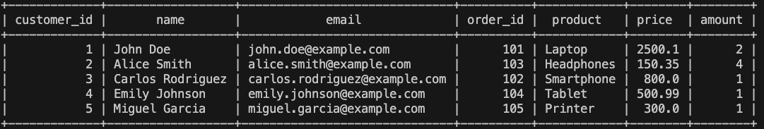
Finally, we check if the information stored in BigQuery is correct:
- Table customer:
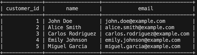
- Tabla sales:
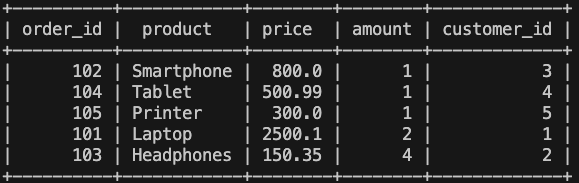
- Final table:
This way, we have managed to have a fully operational functional process through natural language. There is another example that can be executed, although I also encourage creating more examples, or even improving the prompt, to incorporate more complex examples and also adapt it to your use case.
Conclusions and Recommendations
As the examples are very specific to particular technologies, any change in the prompt in any example can affect the results, or also modifying any word in the input request. This means that the prompt is not robust enough to assimilate different expressions without affecting the generated code. To have a productive prompt and system, more training and different variety of solutions, requests, expressions, etc., are needed. With all this, we will finally be able to have a first version to present to our business user so that they can be autonomous.
Specifying the maximum possible detail to an LLM is crucial for obtaining precise and contextual results. Here are several tips to keep in mind to achieve appropriate results:
- Clarity and Conciseness:
- Be clear and concise in your prompt, avoiding long and complicated sentences.
- Clearly define the problem or task you want the model to address.
- Specificity:
- Provide specific details about what you are looking for. The more precise you are, the better results you will get.
- Variability and Diversity:
- Consider including different types of examples or cases to assess the model’s ability to handle variability.
- Iterative Feedback:
- If possible, iterate on your prompt based on the results obtained and the model’s feedback.
- Testing and Adjustment:
- Before using the prompt extensively, test it with examples and adjust as needed to achieve desired results.
Future Perspectives
In the field of LLMs, future lines of development focus on improving the efficiency and accessibility of language model implementation. Here are some key improvements that could significantly enhance user experience and system effectiveness:
1. Use of different LLM models:
The inclusion of a feature that allows users to compare the results generated by different models would be essential. This feature would provide users with valuable information about the relative performance of the available models, helping them select the most suitable model for their specific needs in terms of accuracy, speed, and required resources.
2. User feedback capability:
Implementing a feedback system that allows users to rate and provide feedback on the generated responses could be useful for continuously improving the model’s quality. This information could be used to adjust and refine the model over time, adapting to users’ changing preferences and needs.
3. RAG (Retrieval-augmented generation)
RAG (Retrieval-augmented generation) is an approach that combines text generation and information retrieval to enhance the responses of language models. It involves using retrieval mechanisms to obtain relevant information from a database or textual corpus, which is then integrated into the text generation process to improve the quality and coherence of the generated responses.
Links of Interest
Cloud Storage[1]: https://cloud.google.com/storage/docs
BigQuery[2]: https://cloud.google.com/bigquery/docs
Terraform[3]: https://developer.hashicorp.com/terraform/docs
PySpark[4]: https://spark.apache.org/docs/latest/api/python/index.html
Dataproc[5]: https://cloud.google.com/dataproc/docs
Codey[6]: https://cloud.google.com/vertex-ai/generative-ai/docs/model-reference/code-generation
VertexAI[7]: https://cloud.google.com/vertex-ai/docs
GitHub[8]: https://github.com/alfonsozamorac/etl-genai